Visualizing Geospatial Data in Python Using Folium
Posted by Aly Sivji in Data Analysis
Summary
- Use Python to display location data on interactive map
- Cluster points in a heatmap to visualize usage
One of my favorite things about the Python programming language is that I can always import a library to do the heavy lifting and focus my attention on application logic. It's a testament to the community that so many people are willing to put in the time to create a package and make it easier for other people to get started.
As of this writing, there are around 100,000 packges on PyPI. In this series I call "Exploring PyPI", we will highlight some of the best packages and hidden gems of PyPI.
This post will focus on Folium, the Python interface to the Leaflet JavaScript mapping library. I will explore some of the features of Folium by analyzing data shared by the the City of Chicago's Bike Share system, Divvy.
Divvy Bikes came to Chicago in 2013 and celebrated their ten millionth trip in early 2017. There are stations located all over the city and you can get a 1 day pass for $10 or a yearly membership for $100. Each time you check out a bike, you have 30 minutes to return it to any station before late fees apply. You can check out as many 30 minute blocks as your pass permits.
What You Need to Follow Along
Development Tools (Stack)
- Python 3
- PyData stack (Pandas, matplotlib, seaborn)
- Folium
Code
Setting Up Environment
import folium
from folium import plugins
import pandas as pd
import matplotlib.pyplot as plt
import seaborn as sns

%matplotlib inline
Downloading Data
!wget "https://s3.amazonaws.com/divvy-data/tripdata/Divvy_Trips_2016_Q3Q4.zip"
!mkdir data
!mv Divvy_Trips_2016_Q3Q4.zip data/Divvy_Trips_2016_Q3Q4.zip
!unzip data/Divvy_Trips_2016_Q3Q4.zip -d data/Divvy_Trips_2016_Q3Q4
Directory structure should look like:
.
├── 1-create-divvy-station-heatmap.ipynb
├── README.md
└── data
    ├── Divvy_Trips_2016_Q3Q4
    │   ├── Divvy_Stations_2016_Q3.csv
    │   ├── Divvy_Stations_2016_Q4.csv
    │   ├── Divvy_Trips_2016_Q3.csv
    │   ├── Divvy_Trips_2016_Q4.csv
    │   ├── README_2016_Q3.txt
    │   └── README_2016_Q4.txt
    └── Divvy_Trips_2016_Q3Q4.zip
Loading Data into Pandas
divvyStations_q3 = pd.read_csv('data/Divvy_Trips_2016_Q3Q4/Divvy_Stations_2016_Q3.csv')
divvyStations_q4 = pd.read_csv('data/Divvy_Trips_2016_Q3Q4/Divvy_Stations_2016_Q4.csv')

# combine and keep the first instance of id
divvyStations = pd.concat([divvyStations_q3, divvyStations_q4], axis=0).drop_duplicates(subset=['id'])

divvyStations.head()
| id | name | latitude | longitude | dpcapacity | online_date | |
|---|---|---|---|---|---|---|
| 0 | 456 | 2112 W Peterson Ave | 41.991178 | -87.683593 | 15 | 5/12/2015 |
| 1 | 101 | 63rd St Beach | 41.781016 | -87.576120 | 23 | 4/20/2015 |
| 2 | 109 | 900 W Harrison St | 41.874675 | -87.650019 | 19 | 8/6/2013 |
| 3 | 21 | Aberdeen St & Jackson Blvd | 41.877726 | -87.654787 | 15 | 6/21/2013 |
| 4 | 80 | Aberdeen St & Monroe St | 41.880420 | -87.655599 | 19 | 6/26/2013 |
Using Folium to Visualize Station Data
m = folium.Map([41.8781, -87.6298], zoom_start=11)
m
# mark each station as a point
for index, row in divvyStations.iterrows():
    folium.CircleMarker([row['latitude'], row['longitude']],
                        radius=15,
                        popup=row['name'],
                        fill_color="#3db7e4", # divvy color
                       ).add_to(m)
# convert to (n, 2) nd-array format for heatmap
stationArr = divvyStations[['latitude', 'longitude']].as_matrix()

# plot heatmap
m.add_children(plugins.HeatMap(stationArr, radius=15))
m
Load Divvy Activity Files and Analyze Same Station Rides
The Divvy activity files are split by quarters. We want to concatenate the result of multiple calls to pd.read_csv() so let's be Pythonic and use generators. I adapted a solution I found on Stack Overflow. (Praise Be)
divvyTripFiles = ['data/Divvy_Trips_2016_Q3Q4/Divvy_Trips_2016_Q3.csv',
                  'data/Divvy_Trips_2016_Q3Q4/Divvy_Trips_2016_Q4.csv']

divvyTrips = (pd.read_csv(f) for f in divvyTripFiles)
divvyTripsCombined = pd.concat(divvyTrips, ignore_index=True)

divvyTripsCombined.describe(include='all')
| trip_id | starttime | stoptime | bikeid | tripduration | from_station_id | from_station_name | to_station_id | to_station_name | usertype | gender | birthyear | |
|---|---|---|---|---|---|---|---|---|---|---|---|---|
| count | 2.125643e+06 | 2125643 | 2125643 | 2.125643e+06 | 2.125643e+06 | 2.125643e+06 | 2125643 | 2.125643e+06 | 2125643 | 2125643 | 1590189 | 1.590343e+06 |
| unique | NaN | 1846706 | 1779098 | NaN | NaN | NaN | 584 | NaN | 584 | 3 | 2 | NaN |
| top | NaN | 8/28/2016 13:34:22 | 7/23/2016 12:54:37 | NaN | NaN | NaN | Streeter Dr & Grand Ave | NaN | Streeter Dr & Grand Ave | Subscriber | Male | NaN |
| freq | NaN | 7 | 17 | NaN | NaN | NaN | 59247 | NaN | 64948 | 1589954 | 1180122 | NaN |
| mean | 1.169926e+07 | NaN | NaN | 3.251980e+03 | 1.008547e+03 | 1.799161e+02 | NaN | 1.803518e+02 | NaN | NaN | NaN | 1.980787e+03 |
| std | 7.313875e+05 | NaN | NaN | 1.730437e+03 | 1.816103e+03 | 1.305240e+02 | NaN | 1.304878e+02 | NaN | NaN | NaN | 1.075399e+01 |
| min | 1.042666e+07 | NaN | NaN | 1.000000e+00 | 6.000000e+01 | 2.000000e+00 | NaN | 2.000000e+00 | NaN | NaN | NaN | 1.899000e+03 |
| 25% | 1.106635e+07 | NaN | NaN | 1.755000e+03 | 4.160000e+02 | 7.500000e+01 | NaN | 7.500000e+01 | NaN | NaN | NaN | 1.975000e+03 |
| 50% | 1.170150e+07 | NaN | NaN | 3.446000e+03 | 7.160000e+02 | 1.570000e+02 | NaN | 1.570000e+02 | NaN | NaN | NaN | 1.984000e+03 |
| 75% | 1.233129e+07 | NaN | NaN | 4.802000e+03 | 1.195000e+03 | 2.680000e+02 | NaN | 2.720000e+02 | NaN | NaN | NaN | 1.989000e+03 |
| max | 1.297923e+07 | NaN | NaN | 5.920000e+03 | 8.636500e+04 | 6.200000e+02 | NaN | 6.200000e+02 | NaN | NaN | NaN | 2.000000e+03 |
# Three usertypes? This wasn't mentioned in the readme. Let's investigate
divvyTripsCombined.groupby('usertype')['trip_id'].agg(len)
usertype
Customer       535649
Dependent          40
Subscriber    1589954
Name: trip_id, dtype: int64
## There is a 'Dependent' usertype with 40 entries, let's drop this
divvyTripsCombined = divvyTripsCombined[divvyTripsCombined.usertype != 'Dependent']

# How many trips went from Station A all the way to Station A
totalTrips = len(divvyTripsCombined)
sameStationTrips = divvyTripsCombined[divvyTripsCombined.from_station_id == divvyTripsCombined.to_station_id]
sameStationTrips.is_copy = False

totalTrips = len(divvyTripsCombined)
sameStationTrips = divvyTripsCombined[divvyTripsCombined.from_station_id == divvyTripsCombined.to_station_id]
sameStationTrips.is_copy = False

print ('Total number of trips: {:,}'.format(totalTrips))
print (('Trips from A -> A: {:,}').format(len(sameStationTrips)))
print (('Trips from A -> A: {:.1%}').format(len(sameStationTrips) / totalTrips))
Total number of trips: 2,125,603
Trips from A -> A: 73,730
Trips from A -> A: 3.5%
# % of same station trips by usertype
num_trips_by_usertype = divvyTripsCombined.groupby('usertype')['trip_id'].agg(len)
num_same_station_trips_by_usertype = sameStationTrips.groupby('usertype')['trip_id'].agg(len)
num_same_station_trips_by_usertype / num_trips_by_usertype
usertype
Customer      0.090636
Subscriber    0.015838
Name: trip_id, dtype: float64
This seems like a pretty high percentage of rides to me. Let's look into this a bit more:
- How long are these trips? Accidental checkouts?
- Who is taking them?
- Where are they taking them to?
- Tourists who don't know where the next station is? Or subscribers running errards around the neighbourhood?
- Can we draw conclusions?
sameStationTrips['tripInMinutes'] = sameStationTrips['tripduration'] / 60
sameStationTrips.describe()
| trip_id | bikeid | tripduration | from_station_id | to_station_id | birthyear | tripInMinutes | |
|---|---|---|---|---|---|---|---|
| count | 7.373000e+04 | 73730.000000 | 73730.000000 | 73730.000000 | 73730.000000 | 25204.000000 | 73730.000000 |
| mean | 1.151064e+07 | 3219.399769 | 2360.523261 | 192.533473 | 192.533473 | 1980.622798 | 39.342054 |
| std | 6.886428e+05 | 1731.021515 | 4078.805054 | 153.248962 | 153.248962 | 11.690790 | 67.980084 |
| min | 1.042666e+07 | 1.000000 | 60.000000 | 2.000000 | 2.000000 | 1900.000000 | 1.000000 |
| 25% | 1.091862e+07 | 1716.000000 | 504.000000 | 69.000000 | 69.000000 | 1974.000000 | 8.400000 |
| 50% | 1.144692e+07 | 3395.000000 | 1383.000000 | 164.000000 | 164.000000 | 1985.000000 | 23.050000 |
| 75% | 1.205419e+07 | 4764.000000 | 2888.000000 | 291.000000 | 291.000000 | 1989.000000 | 48.133333 |
| max | 1.297922e+07 | 5919.000000 | 86365.000000 | 620.000000 | 620.000000 | 2000.000000 | 1439.416667 |
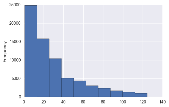
# check out trip in minutes distrubtion
tripDuration = sameStationTrips['tripInMinutes']
tripDuration[tripDuration < tripDuration.quantile(.95)].plot(kind='hist')
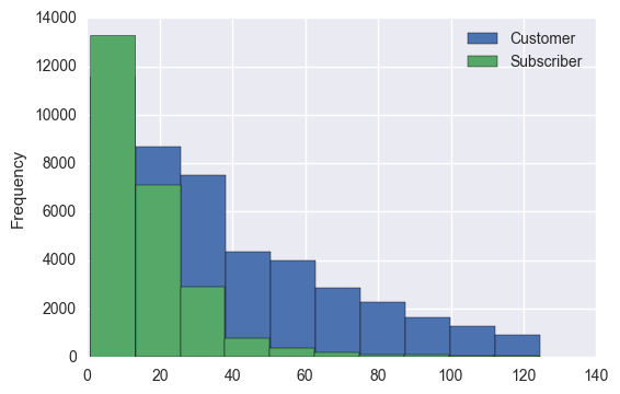
# distribution grouped by subscriber type
sameStationTrips[tripDuration < tripDuration.quantile(.95)] \
  .groupby('usertype')['tripInMinutes'].plot(kind='hist', stacked=True, legend=True)
# Divvy's charge more for rides larger than 30 minutes so lets see that
# distribution of usage for less than 30
sameStationTrips[sameStationTrips['tripInMinutes'] < 30] \
    .groupby('usertype')['tripInMinutes'] \
    .plot(kind='hist', stacked=True, legend=True, bins=20)
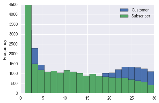
There seems to be a lot of same station trips < 3 minutes. A three minute station to station trip probably implies a mistaken bicycle checkout. Let's go ahead and exclude rides that are less than 3 minutes and see how the distribution looks.
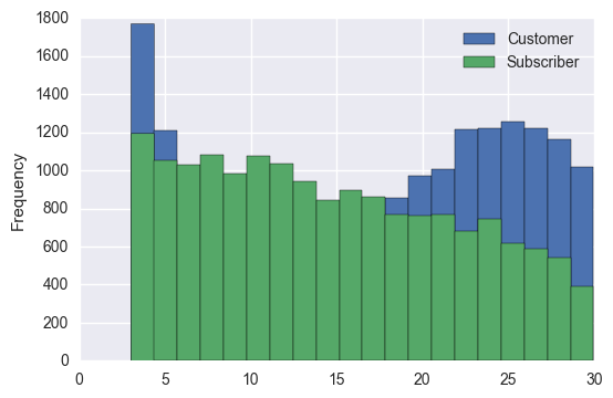
old_count = len(sameStationTrips)
sameStationTrips = sameStationTrips[sameStationTrips.tripInMinutes > 3]
new_count = len(sameStationTrips)
print ('Num records dropped: {}'.format(old_count-new_count))
Num records dropped: 9398
# examine the <30 minute ride distribution again
sameStationTrips[sameStationTrips['tripInMinutes'] < 30] \
    .groupby('usertype')['tripInMinutes'] \
    .plot(kind='hist', stacked=True, legend=True, bins=20)
# Acording to Folium docs, we can pass the heatmap function a (n, 3) ndarray
# with weights in the column
sameStationCountsByStationID = sameStationTrips.groupby('from_station_id')['trip_id'].agg('count')
sameStationCountsByStationID.name = 'numTrips'
sameStationCountsDF = pd.merge(left=divvyStations, right=sameStationCountsByStationID.to_frame(), how='outer',
                               left_on='id', right_index=True)
sameStationCountsDF['numTrips'] = sameStationCountsDF['numTrips'].fillna(value=0)
sameStationCountsDF.head(2)
| id | name | latitude | longitude | dpcapacity | online_date | numTrips | |
|---|---|---|---|---|---|---|---|
| 0 | 456 | 2112 W Peterson Ave | 41.991178 | -87.683593 | 15 | 5/12/2015 | 6.0 |
| 1 | 101 | 63rd St Beach | 41.781016 | -87.576120 | 23 | 4/20/2015 | 137.0 |
Write Helper Function to Simplify Function Calls
We want to map the data we put together; even though Folium makes this relatively easy, we still spend a lot of time wrangling data.
In his book Effective Python, Brett Slatkin makes a case for creating functions with default keyword arguments specified in the definition:
The first advantage is that keyword arguments make the function call clearer to new readers of the code. With the call remainder(20, 7), it’s not evident which argument is the number and which is the divisor without looking at the implementation of the remainder method. In the call with keyword arguments, number=20 and divisor=7 make it immediately obvious which parameter is being used for each purpose.
The second impact of keyword arguments is that they can have default values specified in the function definition. This allows a function to provide additional capabilities when you need them but lets you accept the default behavior most of the time. This can eliminate repetitive code and reduce noise.
We will create a helper function with default keyword arguments to abstact away Folium's complexity. This leaves us with a simple API we can use going forward.
def map_points(df, lat_col='latitude', lon_col='longitude', zoom_start=11, \
                plot_points=False, pt_radius=15, \
                draw_heatmap=False, heat_map_weights_col=None, \
                heat_map_weights_normalize=True, heat_map_radius=15):
    """Creates a map given a dataframe of points. Can also produce a heatmap overlay

    Arg:
        df: dataframe containing points to maps
        lat_col: Column containing latitude (string)
        lon_col: Column containing longitude (string)
        zoom_start: Integer representing the initial zoom of the map
        plot_points: Add points to map (boolean)
        pt_radius: Size of each point
        draw_heatmap: Add heatmap to map (boolean)
        heat_map_weights_col: Column containing heatmap weights
        heat_map_weights_normalize: Normalize heatmap weights (boolean)
        heat_map_radius: Size of heatmap point

    Returns:
        folium map object
    """

    ## center map in the middle of points center in
    middle_lat = df[lat_col].median()
    middle_lon = df[lon_col].median()

    curr_map = folium.Map(location=[middle_lat, middle_lon],
                          zoom_start=zoom_start)

    # add points to map
    if plot_points:
        for _, row in df.iterrows():
            folium.CircleMarker([row[lat_col], row[lon_col]],
                                radius=pt_radius,
                                popup=row['name'],
                                fill_color="#3db7e4", # divvy color
                               ).add_to(curr_map)

    # add heatmap
    if draw_heatmap:
        # convert to (n, 2) or (n, 3) matrix format
        if heat_map_weights_col is None:
            cols_to_pull = [lat_col, lon_col]
        else:
            # if we have to normalize
            if heat_map_weights_normalize:
                df[heat_map_weights_col] = \
                    df[heat_map_weights_col] / df[heat_map_weights_col].sum()

            cols_to_pull = [lat_col, lon_col, heat_map_weights_col]

        stations = df[cols_to_pull].as_matrix()
        curr_map.add_children(plugins.HeatMap(stations, radius=heat_map_radius))

    return curr_map
Let's test it out:
mapPoints(sameStationCountsDF, plotPoints=True, drawHeatmap=True, heatMapWeightsNormalize=True,
          heatMapWeightsCol='numTrips')
Looks good!
Subscriber vs Customer Heatmaps
sameStationCountsByUserTypeStationID = \
    sameStationTrips[['from_station_id', 'usertype', 'trip_id']] \
    .groupby(('usertype', 'from_station_id'))\
    .agg('count')

selected = 'Customer'
sameStationCountsDF = pd.merge(left=divvyStations, right=sameStationCountsByUserTypeStationID.loc[selected],
                               how='outer', left_on='id', right_index=True)
sameStationCountsDF['numTrips'] = sameStationCountsDF['trip_id'].fillna(value=0)

map_points(sameStationCountsDF, plot_points=False, draw_heatmap=True,
           heat_map_weights_normalize=False, heat_map_weights_col='numTrips', heat_map_radius=9)
selected = 'Subscriber'
sameStationCountsDF = pd.merge(left=divvyStations, right=sameStationCountsByUserTypeStationID.loc[selected],
                               how='outer', left_on='id', right_index=True)
sameStationCountsDF['numTrips'] = sameStationCountsDF['trip_id'].fillna(value=0)

map_points(sameStationCountsDF, plot_points=False, draw_heatmap=True,
           heat_map_weights_normalize=False, heat_map_weights_col='numTrips', heat_map_radius=9)
Conclusion
From the maps above, we can see that day pass customers tend to use stations around Lake Michigan and The Loop (Chicago's downtown). This matches up with what I was expecting: that tourists get on a bike to experience Chicago in a different way before continuing with other parts of their trip.
The annual members, on the other hand, have a usage map that is a bit more spread out to the neighborhoods. This could suggest they are running errand before returning their bike to the station where they retrieved it from. I've used Divvy in this manner to pick up take out from a restaurant outside walking distance.
Next Steps
In a future post, I will demostrate how to create choropleth maps to quicky visualize state/county data.
Comments